LONGITUDINAL ANALYSIS OF SURVEY DATA
|
Subtopics
|
|
Introduction
Most sample surveys involve cross-sectional analysis. That is, they provide us with a snapshot of a sample of a population at a single point in time. Time, however, is itself one of the most important variables in politics. The study of change over time is called longitudinal analysis. Here we will focus on the study of change over time in public opinion and behavior, as measured through sample surveys. Longitudinal analysis of survey data can be subdivided into three types: trend analysis, cohort analysis, and panel studies.
Trend Analysis
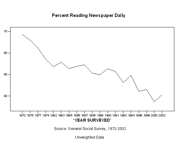
The simplest type of longitudinal analysis of survey data is called trend analysis, which examines overall change over time. This figure, for example, shows how newspaper readership has declined over time:

|
In the first year surveyed, about two-thirds of all respondents reported reading a newspaper on a daily basis. Thereafter, regular newspaper readership more or less continuously declined until, by the start of the new century, only about two respondents in five were daily readers. (Note: look for overall trends, and do not get too caught up in short-term fluctuations. The slight rise in newspaper readership in 2002 could indicate a reversal in the downward trend, but could also be due to short term forces or merely sampling error.)
Trend analysis has some significant limitations. While it can reveal change, it gives us little insight as to how or why the changes have taken place. One possibility is that individuals change their attitudes or behaviors as they move through the life cycle. British Prime Minister Benjamin Disraeli (1804-1881) is supposed to have said that “a man who is not a liberal at 16 has no heart; a man who is not a conservative at 60 has no head.”[1] It may be that people tend to change in predictable ways as they get older (and, depending on one’s perspective, sell out or mature). Another possibility is that people change because of new circumstances. A major crisis, such as a war or depression may result in such changes across all age groups. Changes in technology may have a similar impact. Finally, change may be the result of “generational replacement.” Different generations are shaped by different experiences. Events that occur as people are coming of age are likely to have a big impact on their political outlooks, and this impact may prove lasting, continuing to influence them for the rest of their lives. Even if no individual ever changed after reaching adulthood, overall change would occur as one generation dies out and another generation, having gone through different formative experiences, comes on the scene.
Cohort Analysis
One way to sort some of this out is through cohort analysis. In the examples that will be used here, respondents to the General Social Surveys from 1972 through 2002 have been divided into the following age cohorts:
The GI Generation (born 1927 or earlier — the
earliest year of birth reported by respondents to any of the General Social
Surveys is 1883). Members of this cohort were at least
18 years old by the end of 1945, the year World War II ended.
This generation lived through the Great Depression of the 1930s, the
New Deal, and the Second World War. All Presidents of
the
The Silent Generation (born 1928-1945). This generation came of age after World War II, but before the political turbulence of the late 1960s. The youngest members of the cohort turned 18 the year John Kennedy was assassinated. Because most members reached adulthood in relatively placid times and because it is a relatively small cohort, this group has sometimes been labeled the “silent” generation. At this writing (December 2004), it has yet to produce a president, though three members, Walter Mondale (born 1928), Michael Dukakis (1933), and John Kerry (1943), received major party presidential nominations.
The Baby Boomers (born 1946-1964).
During the Depression and the Second World War, the
Generations X and Y (born after 1964). This cohort includes Generation X (born 1965-1981) and Generation Y (born 1982 or later). The “baby boom” was followed by the “baby bust” as birth rates plummeted in the mid-1960s. Called “Gen X” because, by some reckonings, this is the tenth generation of Americans since independence (hence the Roman numeral “X”), older members of this generation came of age during the administrations of Ronald Reagan and the first President Bush. Younger members attained adulthood during the Clinton Administration. Generation Y (because it comes after Generation X) is sometimes called the “Millennium Generation” because its members came of age (and are still doing so) during or after the year 2000. Members of this cohort will not start to become eligible for the presidency until the 2012 election. In this analysis, Generations X and Y are combined because there are not enough members of the latter group in the voting age population to permit separate analysis.
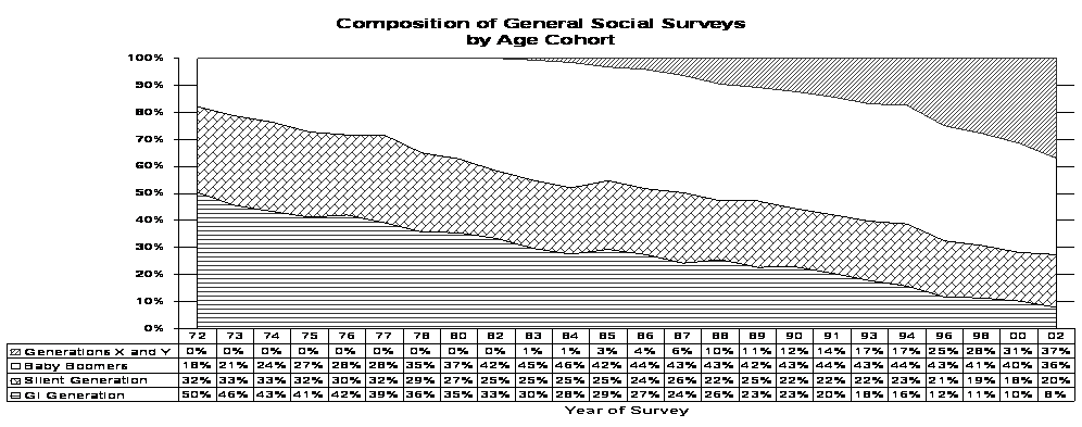
For background purposes, the following figure graphs the changing composition of the General Social Survey from 1972 through 2002.. The same information is presented in tabular form below the graph. The GI Generation provides half of the respondents to the 1972 survey, declining thereafter to less than a tenth of all respondents in 2002. The Silent Generation is a relatively small cohort, never reaching more than about a third of all respondents, and reduced to a fifth in 2002. The Baby Boomers reach their peak of representation in 1984 (46 percent), and still constitute over a third of the total in 2002. The leading edge of Generations X and Y enter the sample in 1983, and by 2002 have become the largest cohort.
 |
As noted earlier, an overall trend, or lack thereof, may be explained in several ways. First may be a new development (a major crisis, or a new technology, for example) that effects all cohorts equally, either suddenly or gradually. If this is the case, trend lines should be similar for each cohort. Second, there may be life cycle factors at work. If Disraeli is correct, an analysis of ideology would show each cohort starting out liberal and gradually becoming more conservative. The trend line for each cohort will be in a conservative direction, but the change for each generation will lag that of the one preceding it. Third, a trend may occur as a result of generational replacement; there may be little within-cohort change over time, but an older generation may pass from the scene and be replaced by a new generation with different attitudes or behaviors. Of course, two or more of these factors may combine to produce the overall pattern.
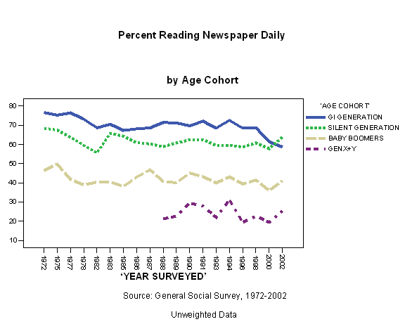
To see how cohort analysis can be applied to study change over time, consider the next figure, which breaks trends in daily newspaper readership down by age cohort. Clearly, the overall trend away from daily newspaper reading is due almost entirely to generational replacement. Habits established early in life seem to persist, but older readers are dying out. Each generation is less devoted to the morning newspaper than its predecessor.

|
While cohort analysis allows us to extract more information from our data than an overall trend analysis, it still suffers from some serious limitations. While people in their twenties who were surveyed in the 1970s are drawn from the same age cohort as people in their 40s interviewed n the 1990s, they are not the same people. Both surveys are subject to random sampling error, and this may produce some of the changes we observe.
Panel Studies
For this reason, the “gold standard” for longitudinal analysis of survey data is the panel study. In a panel, the same people are interviewed at two or more points in time. Since the sample is the same, any changes we observe are not a result of sampling error.
Panel studies, however, have problems of their own. For one thing, they are generally very expensive, since great effort has to be expended to keep track of respondents. For another, despite our best efforts, we will not be successful in all of our attempts to recontact respondents, especially if the study is conducted over a long period of time. Those who drop out of the panel (by moving, dying, refusing to continue, etc.) may have differed in their attitudes and behaviors from those who remain. Finally, there is the problem of reactivity. When respondents are interviewed, their interest in politics may be piqued. If they know that they will be interviewed again, they may even tend to study up on politics so as not to appear ignorant. By the end of the study, what started off as a representative sample may have become something of an elite group.
Optional Exercises
1. Start SPSS, and open “gsscums.sav.” Open the General Social Survey 1972-2002 Subset codebook. Create line charts, repeating the analysis of figures 1 and 3 in this topic, but replacing “news” with another measure of attitude. Is there an overall trend over time? Are there differences within and/or between cohorts? How would you explain the patterns you observe?
The remainder of the exercises for this topic use data from the American National Election Study 2000-2002 Panel Study Subset. Start SPSS, and open “anespanl.sav.” Open the American National Election Study 2000-2002 Panel Study Subset codebook.
2. Even though people may change the way they vote from time to time, they usually do not go back and forth in their party identification, which generally remains stable over time, and even from generation to generation within many families. There is, however, some controversy over how to treat “leaners” (those who initially say that they are independents, but will then acknowledge that they tend to think of themselves as closer to one of the two major parties than the other. Keith et al.[2] argue that leaners are really closet partisans, who think (and vote) much like “weak partisans” (those who initially identify as Democrats or Republicans, but then say that they are “not so strong” in their identification). Others argue that, unlike true partisans, leaners respond to short–term forces. Their “leanings” may give a good indication of how they will vote in this election, but have little long term predictive value.
Test this by doing a crosstab between the seven-point party id measure for 2000 (“ptyid700”) as the independent variable and vote in the 2000 House elections (“house00”) as the dependent variable. Rerun the crosstab, but use vote in the 2002 House elections (“house02”) as the dependent variable. How do leaners compare with partisans?
3. Did some people recall their 2000 president votes differently in 2002 than they had right after the election? Are there any patterns to these changes?
4. The panel study includes feeling thermometers for George W. Bush on the pre and post 2000 election surveys and the pre and post 2002 election surveys. Except for the 2002 post election survey, thermometers are also included for Bill Clinton and Ralph Nader. Compute new variables measuring changes in how respondents felt about each of these people over time. Select independent variables that you think might explain these changes. For example, did Democrats (more than independents and Republicans) become less warm in their feelings toward Ralph Nader as a result of the election? Compare means to test these hypotheses.
For Further Study
Nelson, Elizabeth
N., and Edward E. Nelson, “Research Design and Methods
of Analysis for Change Over Time,”
Palmquist, Ruth A.,
“Survey Methods,”
http://www.gslis.utexas.edu/%7Epalmquis/courses/survey.html.
Accessed
Ruspini,
Elisabetta, “Longitudinal Research in the Social Sciences,”
Social Research Update.
http://www.soc.surrey.ac.uk/sru/SRU28.html.
Spring, 2000. Accessed