CONTINGENCY TABLE ANALYSIS

 

Subtopics Introduction Statistical Significance ·        Chi-square Which Tests Should You Use? Exercises For Further Study

 

Introduction

 

There’s a lot that a contingency table can tell you, if you know the right questions to ask.  How strong is the relationship shown in the table?  What are the odds that the relationship might have occurred just by chance?

 

 

Statistical Significance

 

Doing empirical research involves testing hypotheses suggesting that the value of one variable is related to that of another variable.  If we are working with sample data, we may find that there is a relationship between two variables in our sample, and we wish to know how confident we can be that the relationship is not simply due to chance (or what we call “random sampling error”) but instead reflects a relationship in the population from which the sample was drawn.  How do we go about doing this?

 

If we flip a quarter, the probability of it coming down heads is .5 (or p = .5).  The probability of the quarter coming down heads twice in a row is .5 squared (p = .5² = .25).  For ten heads in a row, p = .5¹⁰ = .0009765, or less than one chance in a thousand.  If we do get ten heads in a row, we will probably conclude that our growing familiarity with the Father of Our Country isn’t just a coincidence, and that there is something wrong with the coin.  Notice what we are doing here.  We aren’t directly testing the idea that the coin is unbalanced.  Instead, we start off with the working assumption that it is balanced.  If our tests show that this is very unlikely, we will reject this assumption. 

 

Similarly, when we wish to test a hypothesis which states that the value of one variable is related to that of another, we begin with the working assumption that the variables are not related.  This working assumption is called the null hypothesis (H_o, pronounced “H sub-naught”).  We then employ techniques (one of which is described below) that tell us the probability that the relationship in our sample has occurred by chance.  If that probability is sufficiently low, we “reject the null hypothesis” and risk concluding that our original hypothesis, oddly referred to by statisticians as the “alternative hypothesis” (H_a), is supported by the data.  In doing so, we have concluded that the relationship is “statistically significant,” and make a “statistical inference” about the population based on the data in the sample.  If, on the other hand, the probability (risk) that the null hypothesis is true is too great, and we conclude that the relationship is not statistically significant, we “fail to reject” the null hypothesis.  This isn’t the same thing as saying that the null hypothesis is true.  It may simply be that we don’t have enough data on which to base a reliable conclusion.

 

The language in the preceding paragraph probably seems rather convoluted.  You’ll get used to it.

 

How low does the probability of the null hypothesis being true have to be before we reject it?  By convention, a null hypothesis is not rejected unless the odds of it being true are less than one in twenty (p < .05).  Of course, it would be even better if the risk were even less, and the odds were less than one in a hundred (p < .01, or “significant at the .01 level”) or one in a thousand (p < .001, or “significant at the .001 level”).

 

Tests for statistical significance assume simple random samples.  While you will rarely be able to work with pure simple random samples, carefully designed studies like the American National Election Study or the General Social Survey come close enough to make the use of such tests reasonable.  Ivory, however, does not come from a rat’s mouth.  If you have a non-probability based sample (such as those discussed in the Data Collection topic) tests for statistical significance won’t bail you out.

 

On the other hand, when you are working with population data (for example, all of the countries in the world or all of the states in the U.S.), you really don’t need tests for statistical significance.  Any relationship you find in your data necessarily applies to the population.  Of course this assumes that your data are otherwise valid.

 

Finally, the fact that a relationship is statistically significant only means that you’ve concluded that there is some relationship between two variables.  It does not necessarily mean that the relationship is a strong one.  To assess that, you need measures of association, an idea to which we will return later in this topic.

 

There are a number of tests for statistical significance that are used for various specific purposes (t-tests, z-tests, F-ratios).  Here we discuss chi-square, a widely used measure of the statistical significance of a relationship between two variables displayed in a crosstabulation

 

 

Chi–square (c²)

 

(There are actually several versions of chi-square.  The most common, and the one we will be using, is "Pearson's chi-square.")

 

Chi-square should be employed when one or both variables are nominal.  If both variables are ordinal or higher, other more powerful tests are appropriate.  

 

Chi-square is used to calculate the probability that a relationship found in a sample between two variables is due to chance (random sampling error).  It does this by measuring the difference between the actual frequencies in each cell of a table and the frequencies one would expect to find if there were no relationship between the variables in the population from which the (simple random) sample has been drawn. The larger these differences are, the less likely it is that they occurred by chance.

 

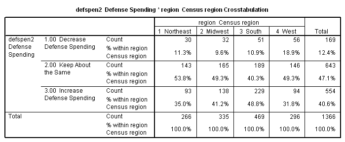
Consider the following table, which shows attitudes toward defense spending broken down by region of the country as measured in the 2000 American National Election Study (with data weighted using the "sample weight" variable).   While our dependent variable (attitude toward defense spending) is ordinal, our independent variable (region) is only nominal.

 

 

The first number in each cell of the table indicates the " count," also called the "observed frequency" because it is the actual number of cases observed in the sample for that cell.  The second number in each cell is the cell count as a percentage of the total number of cases in the column.  We can see that, in the sample, there are some regional differences.  People in the Midwest and South are more likely to favor increasing defense spending than are people in the Northeast and the West, while people in the West are more likely than those in other regions to favor defense spending cuts.   The question is, what are the odds that we would find differences as large as these just by chance, that is, if no regional differences existed in the general population from which the sample was taken (in this case, American adults 18 and older)?

 

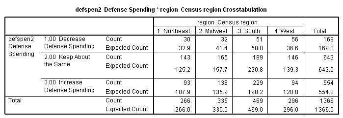
The next table is similar to the first except that the second number in each cell is the "expected frequency," which represents the number of cases we would expect to find in the cell if there were no regional differences.  Note that, for the entire country, we would find that 12.4% of all respondents favored decreasing spending, 47.1% favored the status quo, and 40.5% favored increased spending.  If we apply these percentages within each region, we will (except for rounding error) produce the expected frequencies that make up the second numbers in each cell of the new table.   (In row 1, column 3, for example, 12.4% of 469 equals about 58.  In other words, if the South were just like the rest of the country, we would expect about 58 southern respondents to favor decreased defense expenditures.)

 

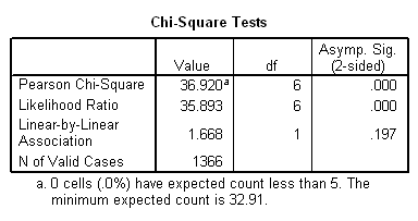
Examine the table and notice that, in some cells there are more cases than the null hypothesis would have led us to expect, while in other cells there are fewer.  Chi-square provides a summary measure of these differences.  In the calculation of chi-square, there are several steps involved [1] .  Differences between observed and expected frequencies (called “residuals”) must be squared (otherwise, they would always add up to zero), then “standardized” to take into account the fact that some cells have larger expected frequencies than others.  For a more detailed explanation of how chi-square is calculated, visit http://davidmlane.com/hyperstat/chi_square.html.  For this table, c² = 36.920.

 

We next need to adjust for the fact that some tables have more cells than others.  We do this by calculating the “degrees of freedom” (d.f.) for the table, which are equal to the number of rows minus 1 times the number of columns minus 1.  In this case, since the table has three rows and four columns, d.f. = (3 – 1)(4 – 1) = 6. 

 

Once we’ve calculated the value of chi-square and determined the degrees of freedom, we can look up the probability that the differences in the sample are due to chance by referring to a table of “critical values of chi-square” found in the appendices of most statistics texts.  Better yet, we can let the computer figure it out for us.  In this case, a chi-square of 36.920 in a table with 6 degrees of freedom would occur by chance less than one time in a thousand (which we would write as “p<.001).”.  The relationship is indeed statistically significant.

 

(In SPSS, “Asymp. Sig.” is equivalent to “p.”  If “Asymp. Sig.” is shown as “.000,” this really means “<.0005,” which SPSS rounds to the nearest thousandth.)   

 

 

 

For Further Study

 

Creative Research Systems,” Statistical Significance,” The Survey Research System: Your Complete Software Solution for Survey Research. http//www.surveysystem.com/signif.htm.   

 

Lane, David M., “Chapter 16: Chi-Square,” HyperStat Textbook Online.  http://davidmlane.com/hyperstat/chi_square.html.