POL242
LAB MANUAL: EXERCISE 10
Logistic Regression
Task
1: Explain support for gay marriage
Task
2: Explain the Canadian Vote
Ordinary Least Squares Regression is inappropriate for explaining dependent
variables that are dichotomous. Look at the example below: all of the
observations are at two places on the Y axis, at one and at zero. This is real
data. The X-axis is the median income of American states. The Y-axis is one if
the state voted for Bush in 2000, zero if the state voted for Gore. To simplify,
I include only the ten poorest states and the ten richest states. As you can
see, almost all of the poorest states (including Mississippi, Arkansas and
Gore's home state, Tennessee) voted for Bush, but most of the rich states voted
for Gore.
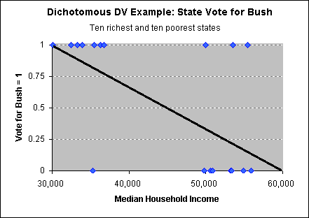 |
When you try to fit any regular,
linear regression line (see chart on right), you cannot do a very good job
of minimizing the errors, so the fit is very poor.
Notice what the line
predicts should be the value of Y for when X=50,000.
A regression line predicts that, for most
levels of X (median income), Y should be between one and zero.
It is also not uncommon for a regression line to
predict values less than zero or higher than one.
Of course, this cannot happen: a state
either votes for Bush (1) or votes for Gore (0). As a result, the
distance between almost all points and the line is quite large. The
distance is even larger for those points that seem to be "wrong" - notice
how far away from the regression line is the point for New Mexico, the
poorest state to vote for Gore (in the bottom-left of the chart).
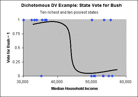
|
Instead, we fit an S-shaped, curved line
to the data (see chart on left). (This line has a negative slope, so it
looks more like a Z, but the positive slope looks more like the letter
S).
This line does a much better job of minimizing the errors. The
band of values of X for which Y should be between one and zero is
minimized. By rounding up values predicted by the S-curve to be over 0.5
(by default) Webstats will tell us how many observations we correctly
predicted. So, we can interpret the data in terms of increasing the odds,
chances or probability that the choice is one (a vote for Bush), rather
than the predicted value for a given level of X. While this interpretation
is less-straightforward, it is more appropriate for modelling dichotomous
choices.
There are two types of similar S-curves used to analyze
these data, logit and probit. The two are very similar.
Here, we will discuss logit analyses. |
 |
We will only discuss modeling choices between dichotomous variables. There
are ways of analyzing more than two choices. We will not be able to discuss
either method in this class, but you should be aware of their existence. These
methods bridge the gap between the smallest number of intervals that regression
lines can be applied to and these dichotomous choice forms. These include
ordered logit (or probit), which basically fits multiple S-curves like
steps on ordinal dependent variables such as the four-point agree-disagree scale
used in the unrecoded gay marriage variable below, and multinomial logit
(or probit) which enables scholars to use categorical dependent variables with
multiple, but unordered variables, like a question that asks whether the
respondent intends to vote for the Liberals, the Conservatives, and the NDP in
Ontario.
The first thing we need to do is recode our dependent variable(s) to make
dichotomous dummy variables. For this data lab, we will use two variables on the
CRIC 2002 study, one that measures support for more immigration, and one that
gauges support for gay marriage.
Immigration Policy
6. Do you think Canada should
accept more, fewer or about the same number of immigrants as we accept
now?
There are three possible
answers (more, fewer, or about the same). We will combine more and about the
same, to gauge support for continuing Canada's [permissive] immigration
policy.
Gay
Marriage
7.
Do you strongly support, support, oppose or strongly oppose allowing gay and
lesbian couples to marry?
There are
four possible answers. To turn this into a dummy variable, we will combine
support and strongly support, and oppose and strongly oppose. A value of one
will indicate support for gay marriage, zero opposition.
***Label! It is important
to make new value labels for any dependent variable when you run a logistic
regression on WebStats or SPSS, as you will see below.***
Example
1: Immigration Policy
Right
click here to open a new window to see the output for the immigration policy
example.
At the top of the page, there 's useful information. You see the
number of cases used in the analysis, so you can make sure you remembered to get
rid fo the missing values. Then you can check that you coded the dependent
variable properly, and it tells you what the dependent variable is (in this
case, the question on support for immigration). All of this is useful, but
little is important or newsworthy. Skip down a few lines and you will see a list
of the independent variables.
|
For this example, I
used:
Q3 Are you worried about you or a member of your
family finding or keeping a stable, full-time job?
Q38 Over the next
decade, do you think that it is likely that we [Canada] will reduce
prejudice against ethnic and racial minorities?
Q42 What is the highest
level of education you have reached?
Q45 Total annual
income
|
I expect that those who are worried
about losing their jobs will be less supportive of admitting immigrants. I also
expect that those who think that Canada will not reduce prejudice against
against ethnic and racial minorities will not support admitting immigrants (most
of whom are minority group members). However, I expect the educated and the
wealthy to support opening the border.
Below the list, there are some
numbers, labeled "goodness of fit," "model chi-square" and others, that for now,
you can disregard. The important information is at the very bottom of the page,
the Classification Table
and the Variables in the
Equation List.
The Variables in the Equation List
should remind you of the multiple regression output. It is very similar. On the
far left, you find a columnar list of variables used in the analysis. Along each
row is information about the size and direction of the coefficient, as well as
whether or not the independent variable is significant.
The third column
from the right, highlighted in blue is labeled "Sig" and indicates the
significance of the variable coefficient. Just like with multiple regressions,
this tells you whether the variable had an effect on the value of Y. If you
observe a number close to 0.000, you can be confident that the independent
variable has a significant effect on the dependent variable. Q38 (reduce
prejudice) and Q42 (education) are clearly significant. Q3 (worried about losing
job) is significant at the less strenuous standard of (p<0.5). With a P= .6390, Q45 (income) is not
significant.
In the second column, you can view a "B" coefficient. This is like
the regression coefficient. Larger numbers reflect a bigger chance per unit
change in the independent variable than smaller numbers. Even though you cannot
interpret the magnitude of the change the same as you would a regression
coefficient, you can tell whether that variable increases the chances of
supporting a permissive immigration policy by looking at sign of the
coefficient. If the coefficient is positive, a high value for the variable
increases the chances of supporting the policy. For example, look at the B for
education, .4161.
As we expected, those who are more educated, support allowing more or the same
number of immigrants. In contrast, the negative coefficient for Q3, -.1430, indicates that the
more the respondent is worried about losing their jobs, the more likely the
respondent will support decreasing the number of immigrants to
Canada.
Above the Variables in the Equation List
is the Classification
Table. The columns show the predicted Ys, while the rows are the actual,
observed Y in the data. Each row and each column is labeled according to how the
variable is labeled (which is why it is important to label the dependent
variable). Look at the bottom-right corner: There are 549 observations correctly
predicted to be in favor of a permissive immigation policy. A further 147
observations in the blue cell in the top-left, indicating that these
observations were correctly predicted to be people who think that there should
be fewer immigrants let into the country. The other two cells of this table are
the observations that the model incorrectly predicted. The best models have many
observations in the two blue cells, with few in the red cells. This model
incorrectly classified too many as being in favor of a permissive immigration
policy, when in actuality, they oppose more immigrants.
In total, this
model correctly classified 60.05% of the observations. Good models should be
better than tossing a coin, or 50% of the observations. Good models should also
exceed the naive model. The naive model is the percent of observations explained
if you always guess 'one' or 'zero' (whichever is the most common). Since about
58% of the actual observations are in favor of Canada's immigration policy or
making it more permissive, this model only slightly improves on the naive model.
Above the classification table are some goodness of fit measures. The
Model Chi-Square is useful when comparing models with
a set a variables to another model with the same set of variables, plus a few
more. The difference in chi-squares indicates whether these additional variables
improved the model.
Example 2 and Task 1: Gay marriage
Now it is your
turn. Right
click here to open a new window to see a second example, using Q6, support
or opposition to gay marriage. I have done much of the work for you. At the top
of the page is the syntax to run an analyis using three dependent variables,
level of education, age, and religiosity.
Look at the Variables in the Equation
List.
1) Are all three variables
significant at P <
0.1? P < 0.5?
2) What sign are the coefficients? Which
variable(s) increase the odds of supporting gay marriage? Which variable(s)
decrease the odds?
Look at the Classification Table.
3) What percentage of the
observations did the model correctly predict? Does this percentage exceed the
naive model?
4) Where is the model weak? In other words, where is the model
over-predicting or under-predicting the most numerous observations?
Now,
try to improve the model. Cut and paste this syntax into WebStats so
you can run the existing models. Go to the CRIC 2002 codebook, and add
at least two independent variables to the model, or add one new independent
variable and one interaction term. Try to focus on correcting the model's
biggest weakness. Remember to recode the variables and get rid of missing
values. For those of you who have not worked with this data set before, a
student in last year's class who wrote her final paper on gay marriage, Anna
Saini, suggested that you might have good results if you used two variables from
the following list (but you can try any variables you'd like):
|
Language (French vs.
English)
Gender
Q9 Importance of obedience of authority
Q13
Opinion of Charter
Q15A Opinion about equality
Q15C Entitlement to
legal rights and protection
Q15F Respect for authority
Q16A Charter
goes too far protecting the rights of minority groups
Q45
Income |
After re-running the analysis with
these new variables, answer the following questions:
1) Did
each of the variables you added have a significant effect on support for [or
opposition to] gay marriage?
2) Did high values of your variables increase
the chance of supporting gay marriage, or decrease chance of supporting gay
marriage?
3) How well did your new model do at predicting support for, and
opposition to gay marriage? Did you improve upon the original model?
To
answer this last question, you should look at the Classification Table, but you
can also compare the Model
Chi-Square.
Task 2: Explain the Canadian Vote.
The problem
with the CRIC data is that the number of possible independent variables are
somewhat limited. So, for the second task, turn to another dataset, the CNES
Canadian National Election Survey. As you can see by looking at the codebook
found at http://www.fas.umontreal.ca/pol/ces-eec/ces.html,
there is no shortage of variables in this dataset.
The dependent
variable you will use is A4, the respondent's vote intention. To perform a
logistic regression, you must recode this variable into a dichotomous dummy
variable, with one taking the value of the party of your choice and zero being
all other parties.
Choose at least three independent variables, or two
independent variables and an interaction term. You may find Section M, which
contains demographics, to be especially useful to find independent variables.
Remember to recode turn all unordered categorical variables into dummy
variables. Run a logistic regression. After running the regression, be ready to
answer:
Look at the Variable Equation List.
1) Are all your variables
significant at P < 0.1? P < 0.5?
2) What sign are the coefficients?
Which variable(s) increase the odds of voting for the party of your choice?
Which variable(s) decrease the odds?
Look at the Classification Table.
3) What percentage of the
observations did the model correctly predict? Does this percentage exceed the
naive model?
4) Where is the model weak? In other words, where is the model
over-predicting or under-predicting the most numerous
observations?
Be ready to share your findings with the rest
of the class.